CDesk: 2. scRNA pipeline
Our CDesk scRNA module comprises of 8 function submodules. Here we present you the CDesk scRNA working pipeline and how to use it to analyze your scRNA data.
2.1 scRNA: Preprocess
CDesk preprocess module integrates preprocessing tools for single-cell RNA-seq data and supports four distinct analysis workflows: cellranger, drseq, singleron, and dnbc. Below is a brief overview of each:
- cellranger: The official 10x Genomics pipeline for single-cell RNA-seq analysis. This workflow checks the input CSV file for sample names and FASTQ file paths, creates symbolic links to the cellranger/input directory, and then runs cellranger count for each sample using the specified reference genome.
- singleron: Based on Singleron’s Celescope pipeline. This workflow links FASTQ files to the singleron/data directory, generates a sample mapping file (mapfile), and runs multi-sample analysis using the multi_rna command, followed by execution of the generated shell script.
- dnbc: A single-cell RNA-seq analysis pipeline developed by MGI for the DNBelab C4 platform, powered by dnbc4tools. It requires cDNA and oligo FASTQ files as input and performs data processing using the dnbc4tools rna run command with a user-specified genome index.
- drseq: Use the quality control and analysis software DrSeq for Drop-seq data. It takes two sequencing files as input: data_1.fastq (containing barcode information) and data_2.fastq (containing read sequences).
- smartseq: The preprocess pipeline is the same as bulkRNA preproces.
1. cellranger
Here is an example about how to use the CDesk preprocess cellranger module.
CDesk scRNA preprocess cellranger \
-i /.../input.csv \
-s mm10 -o /.../output_directory
| Parameters(*necessary) | Description | Default value |
|---|---|---|
| -i,--input* | The input fq information file | |
| -o,--output* | The output directory | |
| -s,--species* | Specify the species | |
| -t,--thread | Number of threads | 8 |
If the pipeline runs successfully, there would be a cellranger running output in the output directory.
What should the input file look like?
=== cellranger.csv ===
sample,fq1,fq2
pbmc,/mnt/linzejie/CDesk_test/data/2.scRNA/1.preprocess/10x/pbmc_1.fastq.gz,/mnt/linzejie/CDesk_test/data/2.scRNA/1.preprocess/10x/pbmc_2.fastq.gz

- sample: The sample name to assign as prefix
- fq1: The fastq read1 compressed file
- fq2: The fastq read2 compressed file
2. singleron
Here is an example about how to use the CDesk preprocess singleron module.
CDesk scRNA preprocess singleron \
-i /.../input.csv \
-s mm10 -o /.../output_directory
| Parameters(*necessary) | Description | Default value |
|---|---|---|
| -i,--input* | The input fq information file | |
| -o,--output* | The output directory | |
| -s,--species* | Specify the species | |
| -t,--thread | Number of threads | 8 |
If the pipeline runs successfully, there would be a celescope running output in the output directory.
What should the input file look like?
=== celescope.csv ===
sample,fq1,fq2
D0,/mnt3/linzejie/CDesk_test/data/2.scRNA/singleron/D0_1.fq.gz,/mnt3/linzejie/CDesk_test/data/2.scRNA/singleron/D0_2.fq.gz
D4,/mnt3/linzejie/CDesk_test/data/2.scRNA/singleron/D4_1.fq.gz,/mnt3/linzejie/CDesk_test/data/2.scRNA/singleron/D4_2.fq.gz

- sample: The sample name to assign as prefix
- fq1: The fastq read1 compressed file
- fq2: The fastq read2 compressed file
3. dnbc
Here is an example about how to use the CDesk preprocess dnbc module.
CDesk scRNA preprocess dnbc \
-i /.../input.csv \
-s mm10 -o /.../output_directory
| Parameters(*necessary) | Description | Default value |
|---|---|---|
| -i,--input* | The input fq information file | |
| -o,--output* | The output directory | |
| -s,--species* | Specify the species | |
| -t,--thread | Number of threads | 8 |
If the pipeline runs successfully, there would be a dnbc4tools running output in the output directory.
What should the input file look like?
=== dnbc.csv ===
sample,cDNAfq1,cDNAfq2,oligofq1,oligofq2
PHCAR_Day4,/mnt3/linzejie/CDesk_test/data/2.scRNA/dnbc/huada/PHCAR_Day4_R1_001.fastq.gz,/mnt3/linzejie/CDesk_test/data/2.scRNA/dnbc/huada/PHCAR_Day4_R2_001.fastq.gz,/mnt3/linzejie/CDesk_test/data/2.scRNA/dnbc/huada/PHCAR_Day4-oligo_R1_001.fastq.gz,/mnt3/linzejie/CDesk_test/data/2.scRNA/dnbc/huada/PHCAR_Day4-oligo_R2_001.fastq.gz
PHCAR_Day8,/mnt3/linzejie/CDesk_test/data/2.scRNA/dnbc/huada/PHCAR_Day8_R1_001.fastq.gz,/mnt3/linzejie/CDesk_test/data/2.scRNA/dnbc/huada/PHCAR_Day8_R2_001.fastq.gz,/mnt3/linzejie/CDesk_test/data/2.scRNA/dnbc/huada/PHCAR_Day8-oligo_R1_001.fastq.gz,/mnt3/linzejie/CDesk_test/data/2.scRNA/dnbc/huada/PHCAR_Day8-oligo_R2_001.fastq.

- sample: The sample name to assign as prefix
- cDNAfq1: The cDNA fastq read1 compressed file
- cDNAfq2: The cDNA fastq read2 compressed file
- oligofq1: The oligo fastq read1 compressed file
- oligofq2: The oligo fastq read2 compressed file
4. drseq
Here is an example about how to use the CDesk preprocess drseq module.
CDesk scRNA preprocess drseq \
-i /.../input.csv \
-s mm10 -o /.../output_directory
| Parameters(*necessary) | Description | Default value |
|---|---|---|
| -i,--input* | The input fq information file | |
| -o,--output* | The output directory | |
| -s,--species* | Specify the species | |
| -t,--thread | Number of threads | 8 |
| --barcode | The barcode range | 1:12 |
| --umi | The UMI code range | 13:20 |
If the pipeline runs successfully, there would be a DrSeq running output in the output directory.
What should the input file look like?
=== DrSeq.csv ===
sample,fq1,fq2
pbmc,/mnt/linzejie/CDesk_test/data/2.scRNA/1.preprocess/10x/pbmctest_1.fastq,/mnt/linzejie/CDesk_test/data/2.scRNA/1.preprocess/10x/pbmctest_2.fastq

- sample: The sample name to assign as prefix
- fq1: The fastq read1 compressed file
- fq2: The fastq read2 compressed file
5. smartseq
The same as CDesk bulk preprocess.
2.2 scRNA: cluster
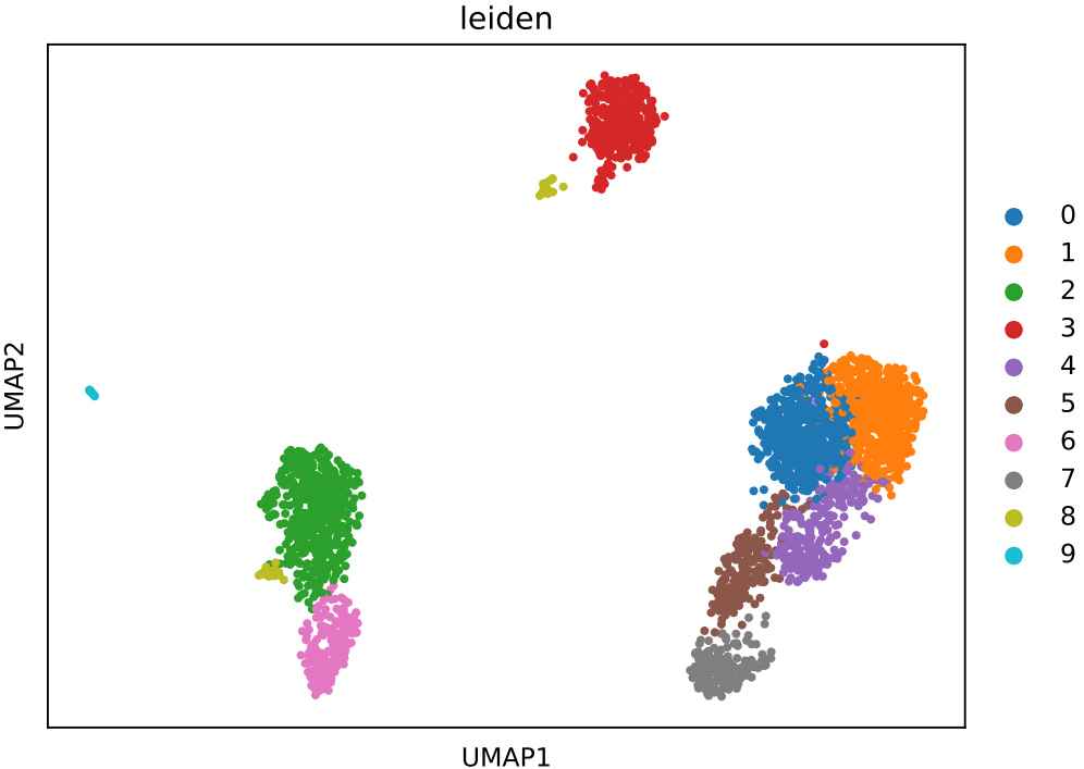
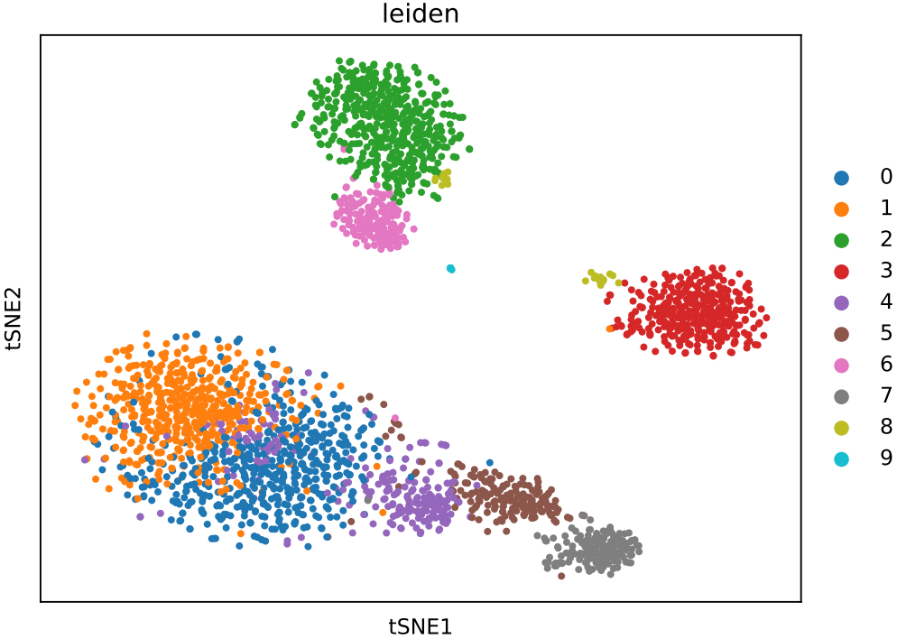
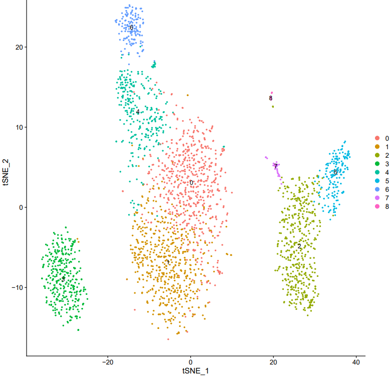
CDesk scRNA cluster module automates scRNA-seq clustering analysis by providing two analytical modes: Seurat (R) and Scanpy (Python). The workflow includes standard scRNA-seq analysis steps—data loading, quality control (filtering of genes and cells, mitochondrial gene content assessment), normalization, feature selection, dimensionality reduction (PCA, UMAP, t-SNE), and clustering. It supports multiple input formats, including H5, H5AD, RDS, and 10x Genomics data, and generates comprehensive PDF reports containing clustering results and visualizations.
Here is an example about how to use the CDesk scRNA clustering module.
CDesk scRNA cluster \
-i /.../input \
-o /.../output_directory \
-n test --mode seurat(scanpy)
| Parameters(*necessary) | Description | Default value |
|---|---|---|
| -i,--input* | The input scRNA data (.h5,.txt/csv/tsv.gz,10x input directory,.rds for seurat mode,.h5ad for scanpy mode) | |
| -o,--output* | The output directory | |
| -n,--name* | The output prefix name | |
| --mode* | Analysis mode | {seurat,scanpy} |
| --min_cells | Genes filtration minimum cells threshold | 3 |
| --min_features | Cells filtration minimum features threshold | 200 |
| --nFeature_RNA_min | cells feature minimum filter threshold | 200 |
| --nFeature_RNA_max | cells feature maximum filter threshold | 2500 |
| --mt_percent | cells mitochondria percent filter threshold | 5 |
| --variable_features | clustering variable features | 2000 |
| --dim_prefer | clustering dimesions | 30 |
| --res | clustering resolution | 1 |
| --width | Plot width | 10 |
| --height | Plot height | 8 |
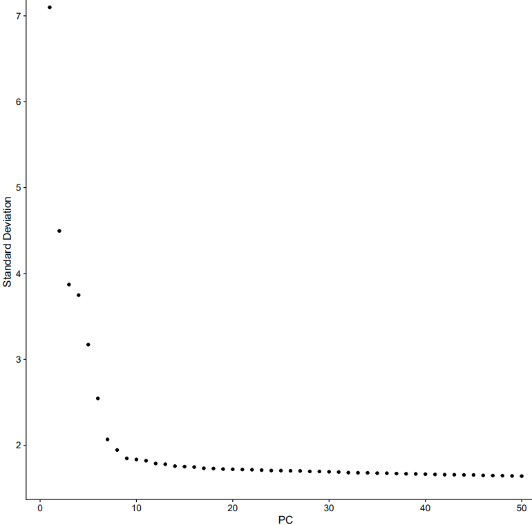
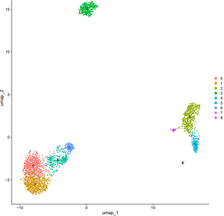
If the pipeline runs successfully, there would be clustering plots and h5ad output file in the output directory for scanpy mode. There would be elbow plots, cluste clustering plots, cluster tree plots and rds output file in the output directory for seurat mode.

2.3 scRNA: annotation
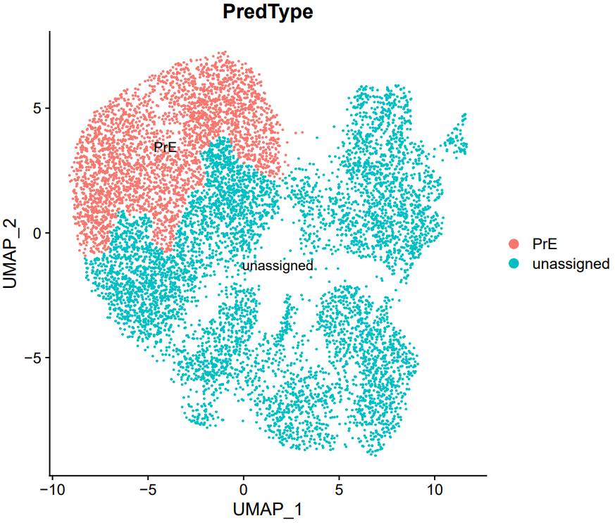
CDesk scRNA annotation module realizes the automation of annotation of single-cell data. It offers two annotation strategies: marker gene-based annotation (marker mode) and reference-guided label transfer (transfer mode). In marker mode, cell types are assigned by comparing the expression levels and detection rates of known marker genes across clusters. In transfer mode, cell type labels from a reference dataset are transferred to the query dataset using Seurat’s integration framework. Both methods produce annotated cell type labels and automatically generate visualizations of the annotations projected onto low-dimensional embeddings.
1. marker mode
Cell type annotation is performed using user-provided marker genes that are specifically associated with defined cell types. Three key thresholds are applied to determine cell type identity:
- The marker gene must have an average expression level in the cluster exceeding the threshold expression_thre (log1p normalized expression).
- The gene must be expressed in a proportion of cells within the cluster greater than percentage_thre.
- For a candidate cell type to be considered, a minimum fraction (marker_percentage) of its marker genes must simultaneously meet both of the above criteria.
Finally, the average proportion score is calculated for each qualifying cell type, and the cell type with the highest score is assigned as the final annotation for each cluster.
Here is an example about how to use the CDesk scRNA annotation marker module.
CDesk scRNA annotation marker \
-i /.../input.rds \
--marker /.../marker.csv \
--meta meta \
-o /.../output_directory
| Parameters(*necessary) | Description | Default value |
|---|---|---|
| -i,--input* | The input .rds file to annotate | |
| -o,--output* | The output directory | |
| --marker* | The marker file with cell marker information | |
| --meta* | The meta colname of reference data used | |
| --cluster | Plot clustering | umap |
| --expression_thre | The average expression threshold | 1.5 |
| --percentage_thre | The express > 0 percentage threshold | 0.7 |
| --marker_thre | The proportion threshold for passing the screening | 0.7 |
| --width | Plot width | 10 |
| --height | Plot height | 8 |
If the pipeline runs successfully, there would be a cell annotation file and a plot of the annotations projected onto low-dimensional embeddings.
What should the input file look like?
=== marker.csv ===
Celltype,Marker
C2,Zscan4a
C2,Zscan4b
C2,Eif1a
C2,Dux
C4,Obox4
C4,Khdc1b
C4,Usp17l1
C4,Zfp352
C8,Cdx2
C8,Pou5f1
C8,Nanog
C8,Eomes
C8,Tead4
TE,Cdx2
TE,Eomes
TE,Gata3
TE,Krt8
TE,Krt18
TE,Elf5
PrE,Gata6
PrE,Gata4
PrE,Sox17
PrE,Pdgfra
PrE,Dab2
PrE,Lrp2

- Celltype: The celltypes to specify
- Marker: The corresponding markers
2. transfer mode
It enables reference-based cell type label transfer. It first loads the reference and query datasets, identifies shared genes, and performs independent preprocessing—including normalization, variable feature selection, scaling, and PCA. Anchors between datasets are then identified using Seurat’s FindTransferAnchors in PCA space, followed by label transfer via TransferData. Cell type annotations from the reference (specified by ref_meta) are predicted and added to the query dataset’s metadata.
Here is an example about how to use the CDesk scRNA annotation transfer module.
CDesk scRNA annotation transfer \
--query /.../qry.rds \
--ref /.../ref.rds \
--meta meta \
-o /.../output_directory
| Parameters(*necessary) | Description | Default value |
|---|---|---|
| --query* | The query .rds data to annotate | |
| --ref* | The reference .rds data | |
| -o,--output* | The output directory | |
| --meta* | The meta colname of reference data used | |
| --cluster | Plot type | umap |
| --nfeatures | The number of variable features | 5000 |
| --dims | The number of PC dimensions used | 30 |
| --width | Plot width | 10 |
| --height | Plot height | 8 |
If the pipeline runs successfully, there would be a cell annotation file and a plot of the annotations projected onto low-dimensional embeddings.
2.4 scRNA: marker
CDesk marker module supports two modes of differential expression analysis for single-cell RNA-seq data:
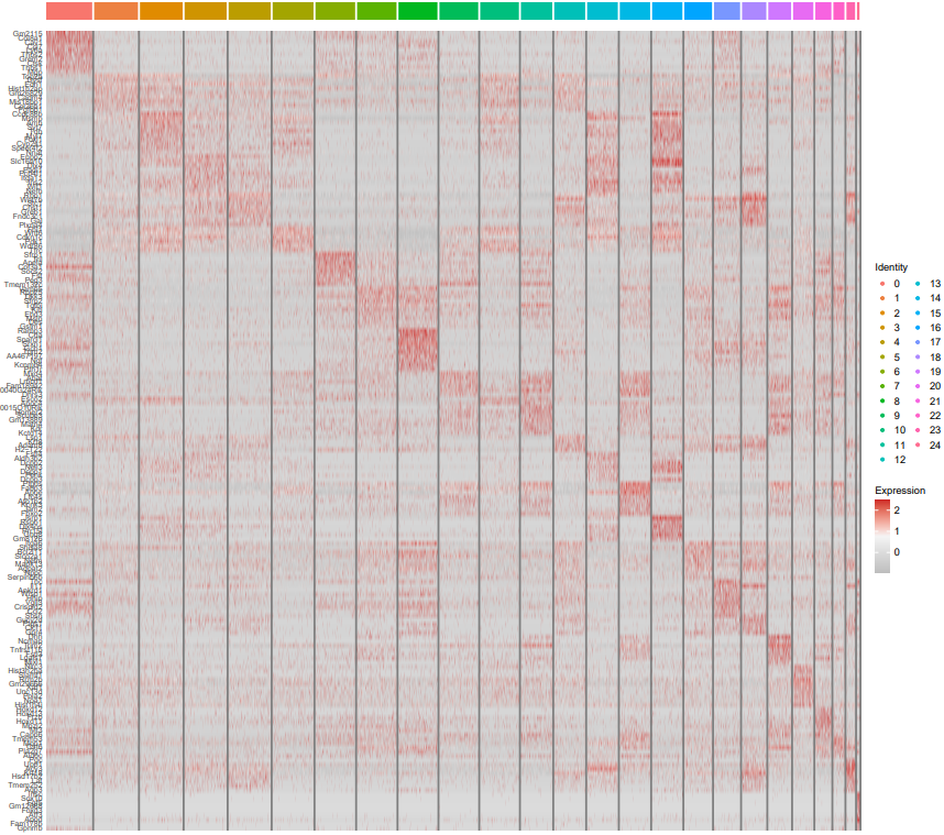
- All-clusters mode (all): Uses FindAllMarkers to automatically identify differentially expressed genes (DEGs) for each cluster compared to all others, and generates a heatmap visualizing the top 10 marker genes per cluster.
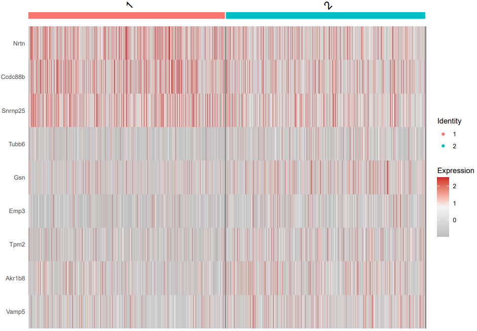
- Two-group mode (2group): Uses FindMarkers to perform pairwise comparison between two user-specified cell types or clusters, identifying their specific DEGs.
Both modes allow customization of key parameters, including log-fold change threshold, adjusted p-value cutoff, and minimum expression percentage. Significantly differentially expressed genes are exported to CSV files for downstream analysis.
1. all
Here is an example about how to use the CDesk scRNA marker all module.
CDesk scRNA marker all \
-i /.../input.rds -o /.../output_directory \
--meta meta -m 0.25 -p 0.05 -f 0.5
| Parameters(*necessary) | Description | Default value |
|---|---|---|
| -i,--input* | The input Seurat object rds file | |
| -o,--output* | The output directory | |
| --meta* | The meta colname of reference data used | |
| -fc | Log Fold Change threshold | 0.5 |
| -p | Adjusted p-value threshold | 0.05 |
| -m | Minimum percentage of expressed cells | 0.25 |
| --width | Plot width | 16 |
| --height | Plot height | 14 |
If the pipeline runs successfully, there would be a cell type marker file and a heatmap plot showing the top differential marker expression in all cell types.
2. 2 group
Here is an example about how to use the CDesk scRNA marker 2group module.
CDesk scRNA marker 2group \
-i /.../input.rds -o /.../output_directory \
--meta meta --type1 type1 --type2 type2 \
-f 0.5 -p 0.05 -m 0.25
| Parameters(*necessary) | Description | Default value |
|---|---|---|
| -i,--input* | The input Seurat object rds file | |
| -o,--output* | The output directory | |
| -m,--meta* | The meta colname of reference data used | |
| --type1* | Specify the first cell type | |
| --type2* | Specify the second cell type | |
| -fc | Log Fold Change threshold | 0.5 |
| -p | Adjusted p-value threshold | 0.05 |
| -m | Minimum percentage of expressed cells | 0.25 |
| --width | Plot width | 16 |
| --height | Plot height | 14 |
If the pipeline runs successfully, there would be a cell type marker file and a heatmap plot showing the marker expression in two cell types.
2.5 scRNA: trajectory
CDesk trajectory module supports four single-cell transcriptomic analysis functions for trajectory inference and RNA velocity:
- cstreet: Performs cell trajectory inference using the CStreet tool.
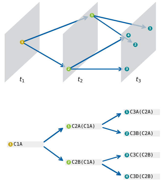
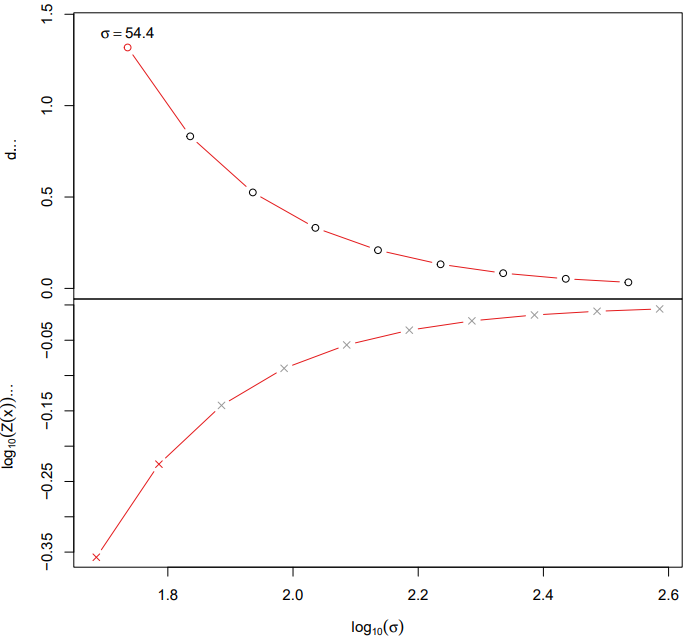
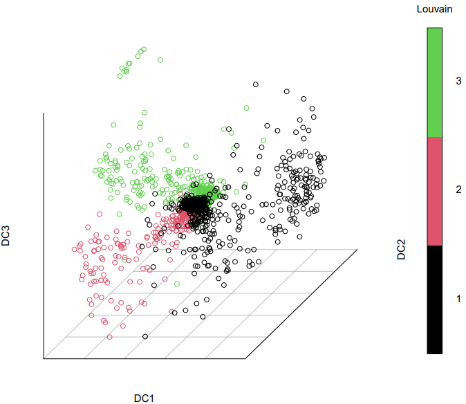
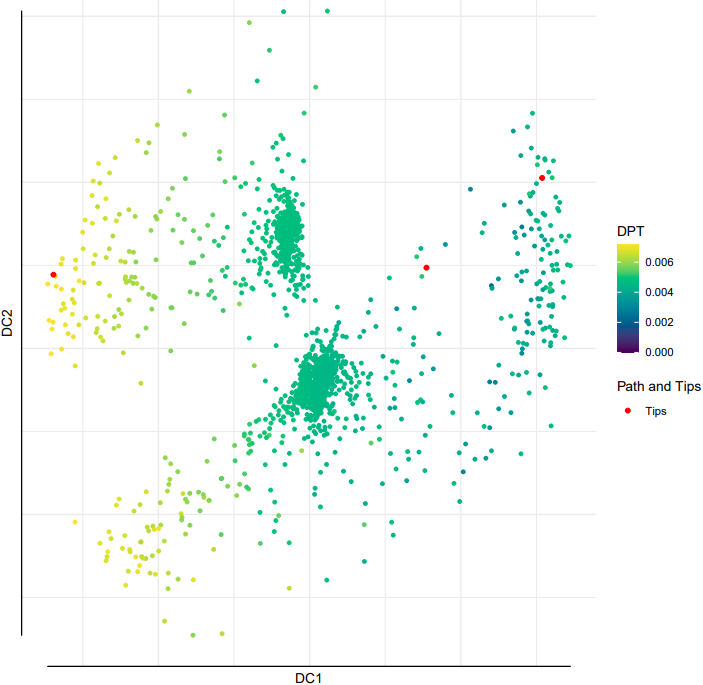
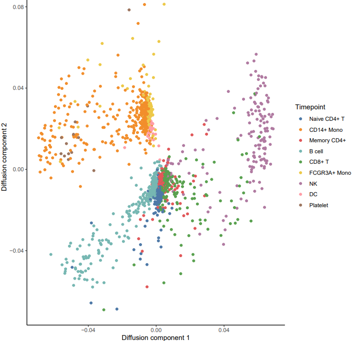
- diffusion: Constructs developmental trajectories via diffusion map embedding and computes pseudotime.
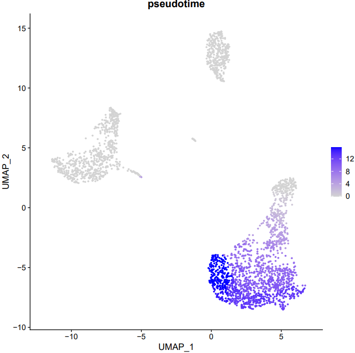
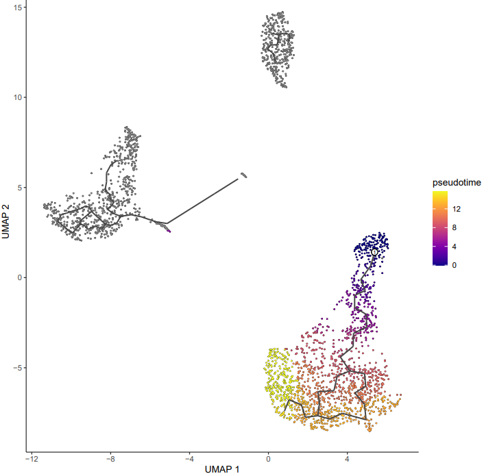
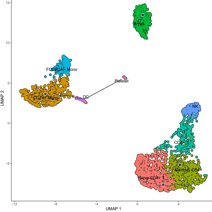
- monocle: Implements advanced trajectory inference with Monocle3, enabling differential gene analysis and co-expression module detection.
- velocity: Conducts RNA velocity analysis to predict cell fate transitions by integrating spliced and unspliced mRNA dynamics, revealing the directionality of cellular state changes.
All modules support parameterized input and generate visual outputs, providing a comprehensive suite for transitioning from static clustering to dynamic developmental analysis of single-cell data.
1. cstreet
Here is an example about how to use the CDesk scRNA trajectory cstreet module.
CDesk scRNA trajectory cstreet \
--expression /.../ExpressionMatrix_list.txt \
--state /.../CellStates_list.txt \
-n test -o /.../output_directory
| Parameters(*necessary) | Description | Default value |
|---|---|---|
| --expression* | Input expression matrixes list file | |
| --state* | Input cell state list file | |
| -o,--output* | The output directory | |
| -n,--name* | The meta colname of reference data used |
If the pipeline runs successfully, there would be CStreet result in the output directory.
2. diffusion
Here is an example about how to use the CDesk scRNA trajectory diffusion module.
CDesk scRNA trajectory diffusion \
-i /.../input.rds \
-o /.../output_directory \
-m meta --start celltype
| Parameters(*necessary) | Description | Default value |
|---|---|---|
| -i,--input* | Input seurat rds file | |
| --start* | Cell type start point for trajectory analysis | |
| -o,--output* | The output directory | |
| -m,--meta* | Meta column for trajectory analysis | |
| --width | Plot width | 8 |
| --height | Plot height | 8 |
If the pipeline runs successfully, it would generate a PDF file containing all diffusion map embeddings and rds object with diffusion map.
3. monocle
Here is an example about how to use the CDesk scRNA trajectory monocle module.
CDesk scRNA trajectory monocle \
i /.../input.rds \
-m meta --start celltype \
-o /.../output_directory
| Parameters(*necessary) | Description | Default value |
|---|---|---|
| -i,--input* | Input seurat rds file | |
| --start* | Cell type start point for trajectory analysis | |
| -o,--output* | The output directory | |
| -m,--meta* | Meta column for trajectory analysis | |
| --width | Plot width | 8 |
| --height | Plot height | 8 |
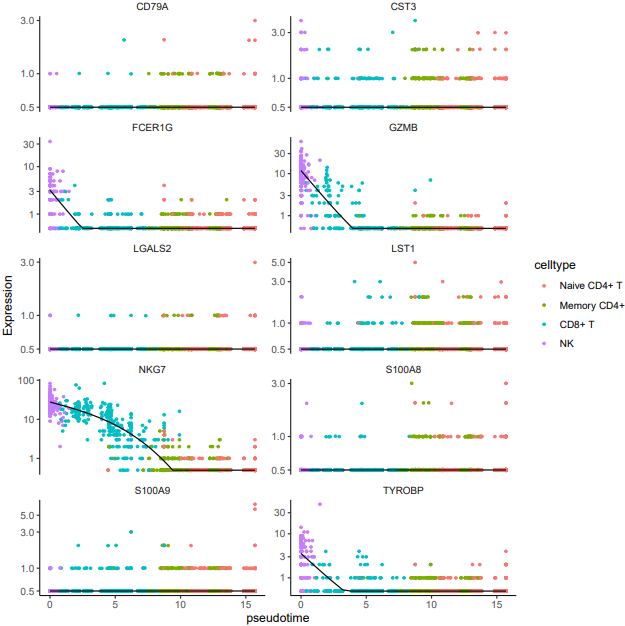
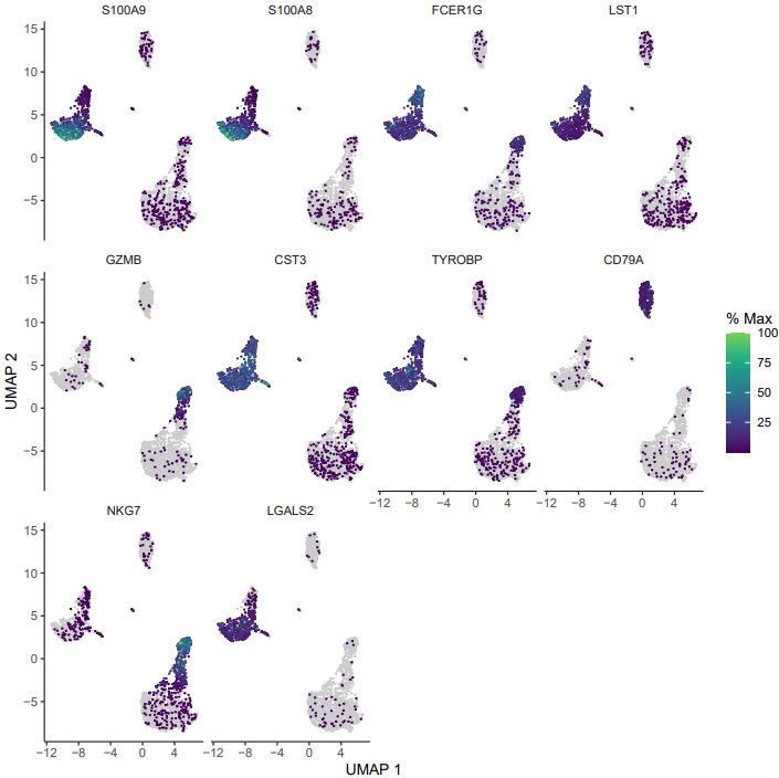
If the pipeline runs successfully, it generates the following outputs:
- Trajectory plot annotated with cell type labels
- Pseudotime trajectory visualization
- Expression trend plots for the top 10 differentially expressed genes
- Feature plots for the top 10 DEGs
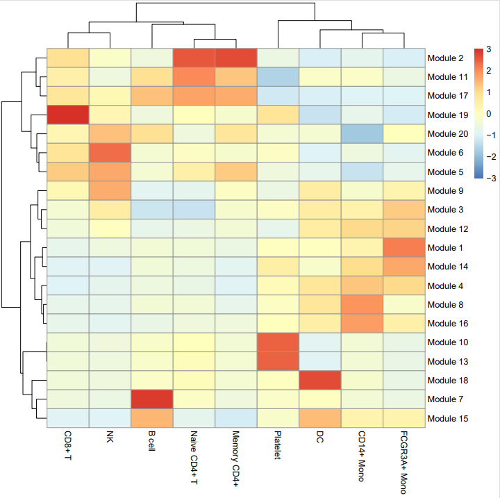
- Co-expression module heatmap
- Seurat object with pseudotime annotations
- Gene module information
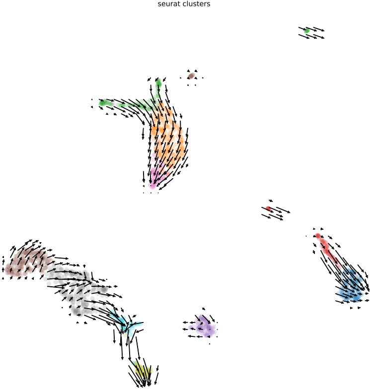
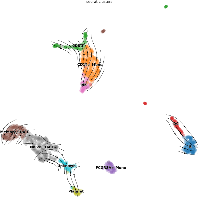
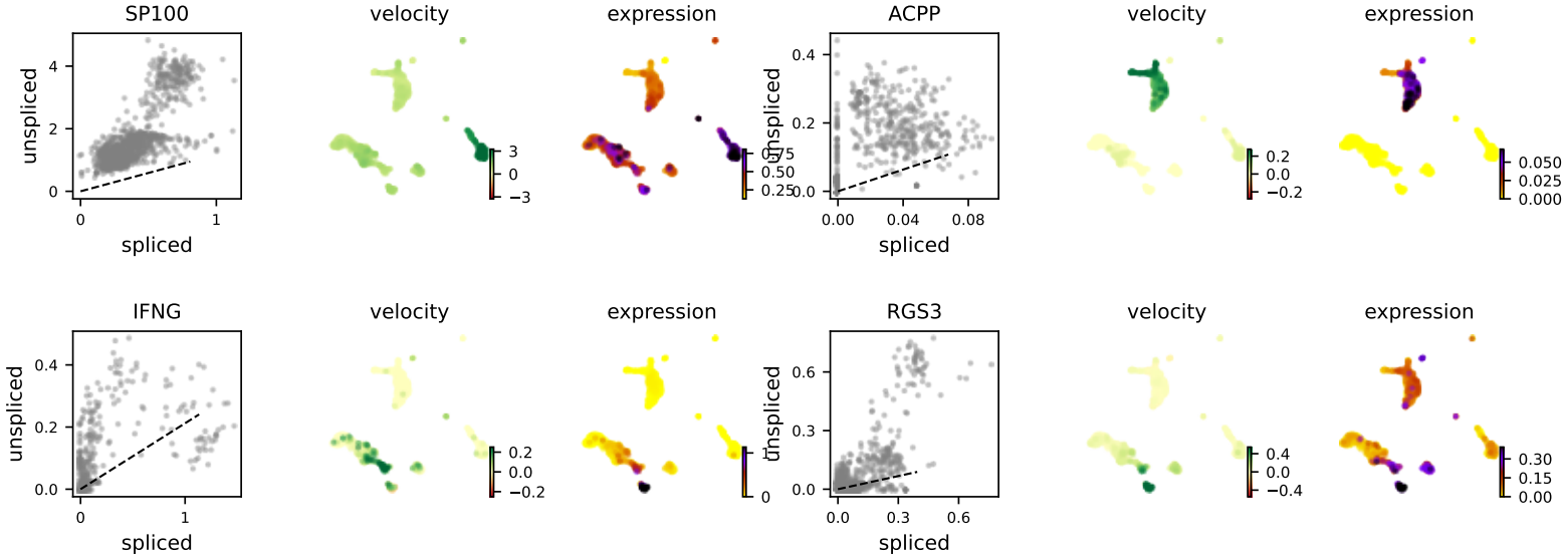
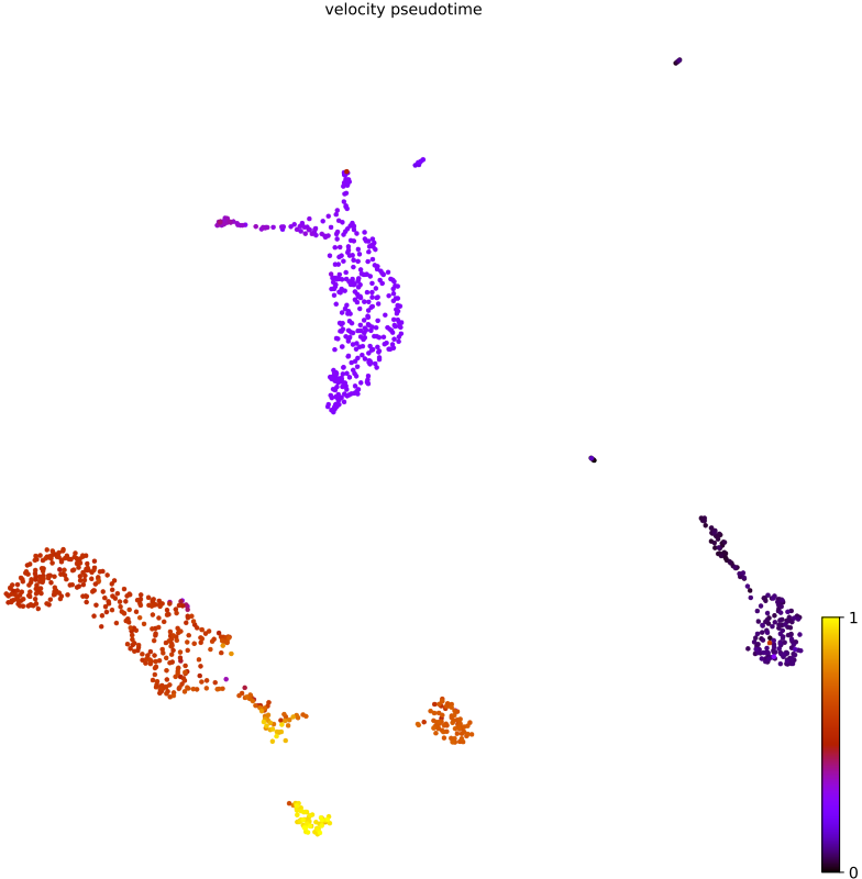
4. velocity
Here is an example about how to use the CDesk scRNA trajectory velocity module.
CDesk scRNA trajectory velocity \
--cellranger /.../cellranger \
--rds /.../input.rds \
--genes /.../genes.txt \
-o /.../output_directory \
--meta meta -s speices
| Parameters(*necessary) | Description | Default value |
|---|---|---|
| --cellranger* | Input cellranger output directory | |
| -s,--species | Specify the species | |
| --rds* | Input seurat rds file | |
| -o,--output* | The output directory | |
| -m,--meta* | Meta column for trajectory analysis | |
| --genes | Interested genes file | |
| -t,--thread | Number of threads | 10 |
| --width | Plot width | 10 |
| --height | Plot height | 10 |
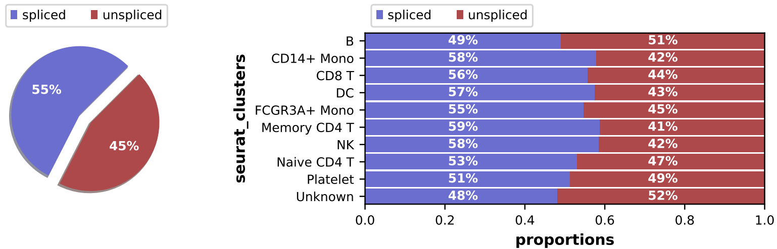
If the pipeline runs successfully, it would generate:
- Loom files generated by velocyto, containing spliced and unspliced count matrices
- Cell IDs, UMAP coordinates, and cluster annotations extracted from the Seurat object
- Bar plots showing the spliced vs. unspliced read ratios for each cluster
- Visualizations of RNA velocity results, including grid velocity and manifold (embedding) plots
- List of identified key genes with significant velocity signals
- Velocity stream plots for user-specified genes of interest (if provided)
- RNA velocity pseudotime plot
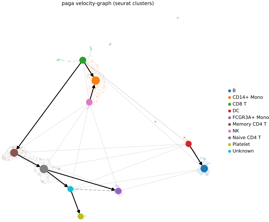
- PAGA (Partition-based Graph Abstraction) graph illustrating the developmental relationships between clusters
2.6 scRNA: similarity
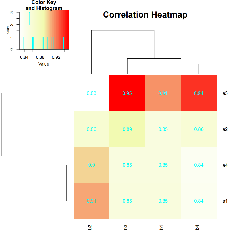
CDesk similarity module assesses gene expression similarity between cell clusters from two single-cell RNA-seq datasets. It supports multiple input formats, reads in both datasets, and performs gene filtering. Using Seurat’s workflow, the module normalizes data, selects highly variable features, and integrates the datasets into a shared embedding space via anchor-based integration. For user-specified pairs of cell clusters, it computes the Pearson correlation coefficient of average gene expression profiles between each cluster pair. The results are visualized as a heatmap annotated with correlation values, enabling intuitive comparison of transcriptional similarity across datasets.
Here is an example about how to use the CDesk scRNA similarity transfer module.
CDesk scRNA similarity \
--sample1 /.../scRNA1 \
--sample2 /.../scRNA2 \
--meta1 meta1 --meta2 meta2 \
--type1 /.../type1.txt \
--type2 /.../type2.txt \
-o /.../output_directory
| Parameters(*necessary) | Description | Default value |
|---|---|---|
| --sample1* | The first scRNA data (.h5,.txt/csv/tsv.gz,10x input directory,.rds for seurat mode,.h5ad for scanpy mode) | |
| --sample2* | The second scRNA data | |
| --meta1* | Meta column used in data 1 | |
| --meta2* | Meta column used in data 2 | |
| --type1* | Data 1 group file | |
| --type2* | Data 2 group file | |
| -o,--output* | The output directory | |
| --nfeatures_used | The number of variable features | 2000 |
| --integrate_features | The number of features for integration | 2000 |
| --width | Plot width | 10 |
| --height | Plot height | 8 |
If the pipeline runs successfully, there would be a correlation heatmap showing the cross-sample cell type similarity analysis in the outputdirectory.
What should the input file look like?
=== type1.txt  ===
a1
a2
a3
a4
=== type2.txt  ===
b1
b2
b3
b4
2.7 scRNA: interaction
CDesk interaction module provides two approaches for analyzing cellular interactions in single-cell data:
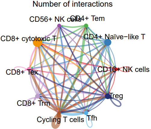
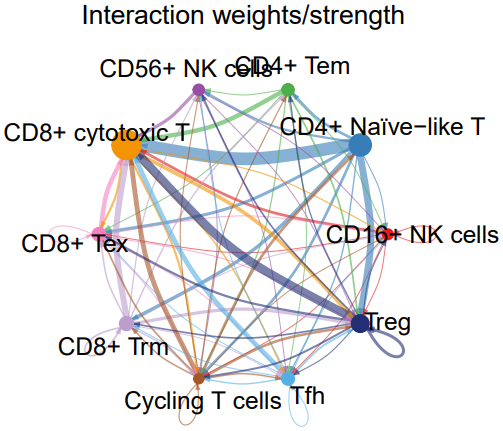
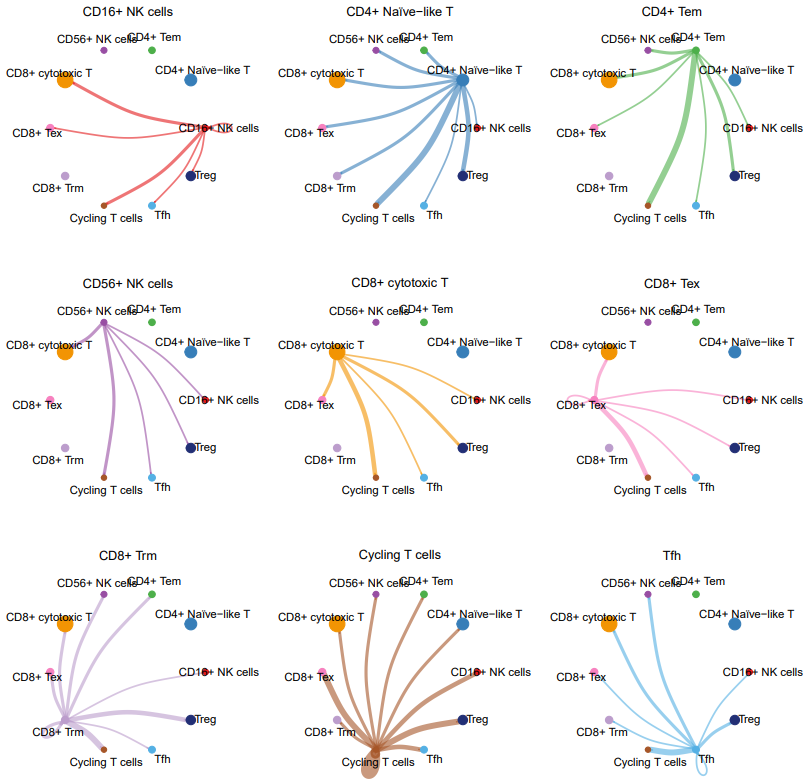
- CellChat: Performs cell-cell communication network analysis by leveraging ligand-receptor interaction databases (CellChatDB). It takes a Seurat object as input, infers signaling probabilities between cell clusters, and reconstructs intercellular communication networks. The method generates visualizations including signaling network graphs, ligand-receptor interaction counts, and signaling strength plots, enabling comprehensive analysis of intercellular crosstalk.
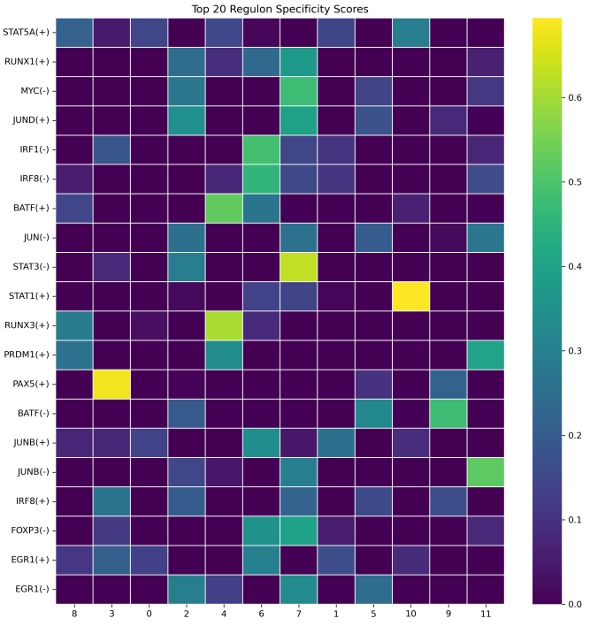
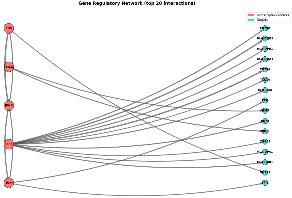
- PySCENIC: Analyzes gene regulatory networks (GRNs) by inferring transcription factor (TF)-target gene co-expression relationships within cells. The pipeline consists of three steps: (1) GRN inference using GRNBoost2, (2) cis-regulatory motif enrichment analysis with RcisTarget, and (3) regulon activity scoring via AUCell. Additionally, it computes Regulon Specificity Scores (RSS) and generates corresponding heatmaps, along with visualizations of the inferred gene regulatory networks.
1. Cellchat
Here is an example about how to use the CDesk scRNA cellchat module.
CDesk scRNA interaction cellchat \
-i /.../input.rds \
-o /.../output_directory \
--s human --group meta
| Parameters(*necessary) | Description | Default value |
|---|---|---|
| -i,--input* | Input Seurat object rds file | |
| -o,--output* | The output directory | |
| -s,--species* | Species (human or mouse) | |
| --group* | Meta column for grouping | |
| -t,--thread | Number of threads | 16 |
| --width | Plot width | 8 |
| --height | Plot height | 8 |
If the pipeline runs successfully, it would generate:
- cellchat.rds: A RDS file containing the complete CellChat object, including all analysis results, which can be reloaded in future R sessions for further exploration.
- net_lr.csv: A CSV file listing ligand-receptor interactions between cell clusters, including ligands, receptors, and interaction strengths.
- net_pathway.csv: This file contains pathway-level interaction information inferred from ligand-receptor pairs.
- cell_net_circle.pdf: A circular plot visualizing the number and strength of interactions between cell clusters.
- TIL_net_number_individual.pdf: A plot showing the number of outgoing signals from each cell cluster when acting as a sender.
- TIL_net_strength_individual.pdf: A plot showing the signaling strength from each cell cluster to others when acting as a sender.
2. Pyscenic
Here is an example about how to use the CDesk scRNA cellchat module.
CDesk scRNA interaction pyscenic \
-i /.../input.data \
-o /.../output_directory \
--tf /.../tfs.txt \
--db /.../db_dir \
--species hg38
| Parameters(*necessary) | Description | Default value |
|---|---|---|
| -i,--input* | Input scRNA file, h5ad/csv/tsv format | |
| -o,--output* | The output directory | |
| --tf* | TF list file | |
| --db* | RcisTarget database directory | |
| -s,--species* | Species (human/mouse/hg*/mm*) | |
| -t,--thread | Number of threads | 16 |
| --auc | AUC threshold | 0.05 |
| --nes | Normalized Enrichment Score threshod | 3 |
| --normalize | Normalize scRNA data or not (True/False) | False |
| --scale | Scale scRNA data or not (True/False) | False |
| --log | Log scRNA data or not (True/False) | False |
| --top_regulons | Show top N regulons | 20 |
| --top_targets | Show top N targets genes for each TF | 20 |
| --plot_tf | Draw network for specific TF |
If the pipeline runs successfully, it would generate:
- adjacencies.csv: The co-expression network results, listing regulatory relationships between transcription factors and target genes with associated weights.
- motifs.csv: Results from cis-regulatory motif enrichment analysis (RcisTarget), identifying significantly enriched motifs and their corresponding regulons.
- scenic_result.loom: A LOOM file containing AUCell scores (regulon activity per cell), suitable for downstream visualization or analysis.
- rss_scores.csv: Regulon Specificity Scores (RSS), indicating the specificity of each regulon across cell types.
- rss_heatmap.png: A heatmap of the top N most cell-type-specific regulons based on RSS.
- grn_network_top.png: A global gene regulatory network (GRN) plot showing the top N highest-weight interactions.
- grn_network_{tf}.png: Individual GRN plots for specific transcription factors (generated only if --plot_tf is specified).
- processed_data.loom (preprocessed data): intermediate files during analysis
What should the input file look like?
=== tfs.txt  ===
BATF
BCL6
EGR1
EGR2
ETS1
FOS
FOXP3
GATA1
GATA3
IRF1
IRF4
IRF8
JUN
JUNB
JUND
LEF1
MYC
NFATC1
NFKB1
NFKB2
PAX5
PRDM1
RELA
RUNX1
RUNX3
STAT1
STAT3
STAT4
STAT5A
=== db_dir  ===
hg38_10kbp_up_10kbp_down_full_tx_v10_clust.genes_vs_motifs.rankings.feather
mm10_10kbp_up_10kbp_down_full_tx_v10_clust.genes_vs_motifs.rankings.feather
motifs-v10nr_clust-nr.hgnc-m0.001-o0.0.tbl
motifs-v10nr_clust-nr.mgi-m0.001-o0.0.tbl
motifs-v9-nr.hgnc-m0.001-o0.0.tbl
motifs-v9-nr.hgnc-m0.001-o0.0.tbl.1
motifs-v9-nr.mgi-m0.001-o0.0.tbl

Genomic region database file (.feather)
Transcription factor motif annotation file (.tbl)
HGNC refers to human gene symbols; MGI refers to mouse gene symbols.
2.8 scRNA: integrate
The integrate module provides two strategies for single-cell data integration: Seurat-based integration and bulk + scRNA-seq integration.
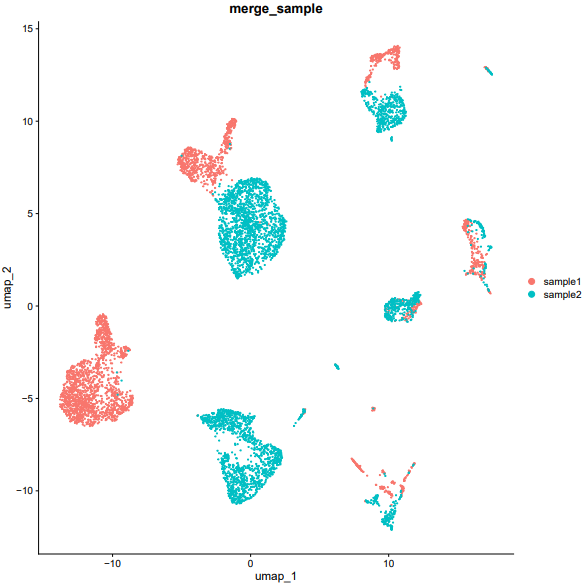
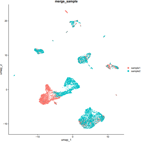
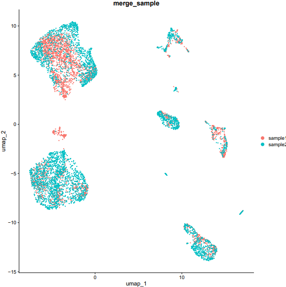
- The Seurat integration mode supports three algorithms—merge, CCA (Canonical Correlation Analysis), and Harmony—to correct batch effects across multiple single-cell datasets, enabling seamless data integration and visualization.
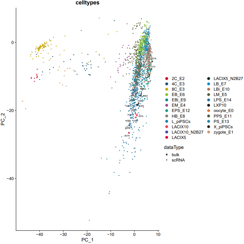
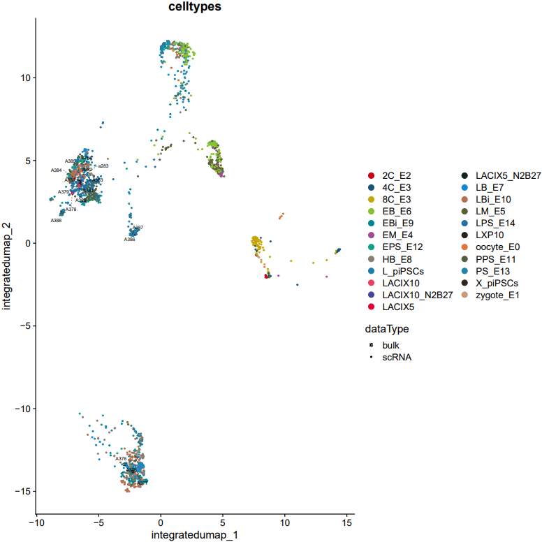
- The bulk + scRNA-seq integration mode innovatively aligns bulk RNA-seq data with single-cell data in a shared gene space, allowing joint visualization in a reduced-dimensional space. This interactive visualization facilitates comparative analysis of the two data types, revealing their relationships and transcriptional similarities.
1. seurat
Here is an example about how to use the CDesk scRNA integrate seurate module.
CDesk scRNA integrate seurat \
-i /.../input.csv \
--mode merge(CCA/harmony) \
-o /.../output_directory
| Parameters(*necessary) | Description | Default value |
|---|---|---|
| -i,--input* | Seurat data list file (multiple formats acceptable) | |
| -o,--output* | The output directory | |
| --mode* | Choose a integration method {merge,harmony,CCA} | |
| --min_cells | minimum cells threshold for data filtration preprocess | 3 |
| --min_features | minimum feature threshold for data filtration preprocess | 200 |
| --nfeatures_used | The number of variable features | 2000 |
| --integrate_features | The number of features for integration | 2000 |
| --pc_num | PCA dimensional reduction dimensions | 50 |
| --pc_reduce | UMAP dimensional reduction dimensions | 30 |
| -max_iter_harmony | Harmony maximal iteration | 20 |
| --k_anchor | k.anchor for CCA integrate | 20 |
| --width | Plot width | 10 |
| --height | Plot height | 10 |
If the pipeline runs successfully, there would be a merged Seurat object and a UMAP plot for batch effect assessment of the integrated data.
What should the input file look like?
=== input.csv  ===
file,group
/mnt/linzejie/CDesk_test/data/2.scRNA/8.integrate/GSM5050521_G1counts.csv.gz,sample1
/mnt/linzejie/CDesk_test/data/2.scRNA/8.integrate/GSM5050523_G2counts.csv.gz,sample2

- Celltype: The celltypes to specify
- Marker: The corresponding markers
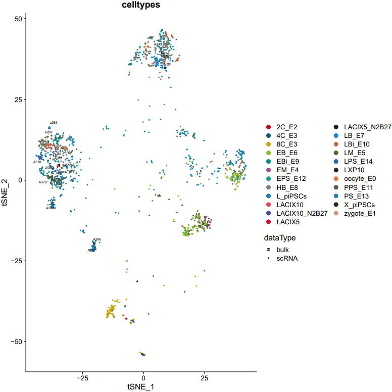
2. bulk
Here is an example about how to use the CDesk scRNA integrate bulk module.
CDesk scRNA integrate bulk \
--bulk /.../bulk_data_list.txt \
--scRNA /.../scRNA_data_list.txt \
--meta /.../meta.csv \
-o /.../output_directory
| Parameters(*necessary) | Description | Default value |
|---|---|---|
| --bulk* | bulkRNA data list file | |
| --scRNA* | scRNA data list file | |
| -m,--meta* | The meta file | |
| -o,--output* | The output directory | |
| --nfeatures_used | The number of variable features | 2000 |
| --integrate_features | The number of features for integration | 2000 |
| --pc_num | PCA dimensional reduction dimensions | 50 |
| --pc_reduce | UMAP dimensional reduction dimensions | 30 |
| --width | Plot width | 10 |
| --height | Plot height | 10 |
If the pipeline runs successfully, there would be a merged Seurat object and and static as well as interactive visualization plots (including PCA, UMAP, and t-SNE) for integrated data.
What should the input file look like?
=== bulk_data_list.txt ===
/mnt/linzejie/CDesk_test/data/2.scRNA/8.integrate/data/GeneSymbol_counts.inhouse.txt
/mnt/linzejie/CDesk_test/data/2.scRNA/8.integrate/data/GeneSymbol_counts.txt
/mnt/linzejie/CDesk_test/data/2.scRNA/8.integrate/data/GeneSymbol_counts.a378_a388.txt
=== scRNA_data_list.txt ===
/mnt/linzejie/CDesk_test/data/2.scRNA/8.integrate/data/GeneSymbol_counts.a4_CRR271345_expmat.txt
/mnt/linzejie/CDesk_test/data/2.scRNA/8.integrate/data/GeneSymbol_counts.a4_CRR271346_expmat.txt
/mnt/linzejie/CDesk_test/data/2.scRNA/8.integrate/data/GeneSymbol_counts.a4_CRR271347_expmat.txt
/mnt/linzejie/CDesk_test/data/2.scRNA/8.integrate/data/GeneSymbol_counts.a4_CRR271348_expmat.txt
/mnt/linzejie/CDesk_test/data/2.scRNA/8.integrate/data/GeneSymbol_counts.a4_CRR271349_expmat.txt
/mnt/linzejie/CDesk_test/data/2.scRNA/8.integrate/data/GeneSymbol_counts.a4_CRR271350_expmat.txt
/mnt/linzejie/CDesk_test/data/2.scRNA/8.integrate/data/GeneSymbol_counts.a4_CRR271351_expmat.txt
/mnt/linzejie/CDesk_test/data/2.scRNA/8.integrate/data/GeneSymbol_counts.a4_CRR271352_expmat.txt
/mnt/linzejie/CDesk_test/data/2.scRNA/8.integrate/data/GeneSymbol_counts.a4_CRR271353_expmat.txt
/mnt/linzejie/CDesk_test/data/2.scRNA/8.integrate/data/GeneSymbol_counts.a4_CRR271354_expmat.txt
/mnt/linzejie/CDesk_test/data/2.scRNA/8.integrate/data/GeneSymbol_counts.a4_CRR271355_expmat.txt
/mnt/linzejie/CDesk_test/data/2.scRNA/8.integrate/data/GeneSymbol_counts.a4_CRR271356_expmat.txt
/mnt/linzejie/CDesk_test/data/2.scRNA/8.integrate/data/GeneSymbol_counts.a4_CRR271357_expmat.txt
/mnt/linzejie/CDesk_test/data/2.scRNA/8.integrate/data/GeneSymbol_counts.a4_CRR271358_expmat.txt
/mnt/linzejie/CDesk_test/data/2.scRNA/8.integrate/data/GeneSymbol_counts.a4_CRR271359_expmat.txt
/mnt/linzejie/CDesk_test/data/2.scRNA/8.integrate/data/GeneSymbol_counts.a4_CRR271360_expmat.txt
/mnt/linzejie/CDesk_test/data/2.scRNA/8.integrate/data/GeneSymbol_counts.a4_CRR271361_expmat.txt
/mnt/linzejie/CDesk_test/data/2.scRNA/8.integrate/data/GeneSymbol_counts.a4_CRR271362_expmat.txt
/mnt/linzejie/CDesk_test/data/2.scRNA/8.integrate/data/GeneSymbol_counts.a4_CRR271363_expmat.txt
/mnt/linzejie/CDesk_test/data/2.scRNA/8.integrate/data/GeneSymbol_counts.a4_CRR271364_expmat.txt
=== meta.csv ===
sample,tag
P1.AAACATCG,2C_E2
P1.AACAACCA,zygote_E1
P1.AACCGAGA,zygote_E1
P1.AACGCTTA,zygote_E1
P1.AACGTGAT,2C_E2
......
A379,LACIX5
A380,LACIX10
A381,LACIX10
A382,LACIX5_N2B27
A383,LACIX5_N2B27
A384,LACIX10_N2B27
A385,LACIX10_N2B27
A386,LXP10
A387,LXP10
A388,LXP10

- sample: The sample(column) name of bulk/scRNA data
- tag: The tag name to specify